Limit of a sequence

Introduction to the limit of a sequence

 Let's consider the sequence:

We can have a graphic representation of this sequence. In order to do that we need to write the sequence as a function i.e  f(n) = n + 1/n². We start by finding the first few points of the graph:

We plug the first values of n in the function in order to find the corresponding values of f(n) 

For n = 1 we have f(1) = 1 + 1/(1)² = 2/1 = 2

For n = 2 we have f(2) = 2 + 1/(2)² = 3/4

For n = 3 we have f(3) = 3 + 1/(3)² = 4/9

For n = 4 we have  f(4) = 4 + 1/(4)² = 5/16

For n = 5 we have f(5) = 5 +1/(5)² = 6/25

The first few points of the graph are: (1, 2), (2, 3/4), (3, 4/9), (4, 5/16), (5, 6/25).

The graph of the function looks like this for the first 30 points of the graph:

 

We observe that as the the value of n increases the value of f(n) decreases. For values of n sufficiently large, aⁿ becomes close to zero. We can express this observation like this:

When n→∞, aⁿ→0. This is nothing than the limit of aⁿ when n approaches infinity. When n approaches infinity the limit of aⁿ is 0. We can express this by the notation: 

Definition of the limit of a sequence

If a sequence aⁿ becomes closer and closer to a number L when the value of n becomes sufficiently large, we say that the limit of  aⁿ is L when n approaches infinity. We write this simply as:

Infinite limit of a sequence

If a sequence aⁿ becomes larger and larger whenever the value of n becomes sufficiently big, we say that the limit of aⁿ is positive infinity when n approaches infinity. We write:

If  aⁿ becomes larger and larger negatively whenever the value of n becomes sufficiently big, we say that the limit of  aⁿ is negative infinity when n approaches infinity. We write:

Precise definition of the limit of a sequence

1) We say that  if for every ε>0 there is an integer N such that

❘aⁿ -L❘＜ε whenever n>M

2) We say that   if for every number M>0 there is an integer N such that

aⁿ >M whenever n>N

3) We affirm that    if for every number M<0 there is an integer N such that

 aⁿ <M whenever n>N

Convergence and Divergence of the limit of a sequence

If the limit of of a sequence when n approaches infinity is a finite number, the sequence is convergent. If the limit of a sequence when n approaches infinity is infinite positively or negatively, the sequence is divergent.

Properties of the limit of a sequence

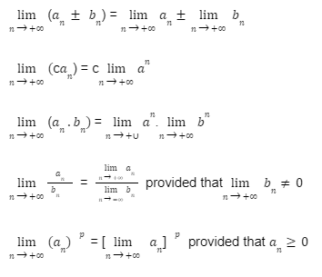
The limit of a sequence is equivalent to the limit of a function since a sequence aⁿ can be written as f(n) = aⁿ. Therefore the properties of the limit of a function are also valid for the limits of a sequence

If aⁿ and bⁿ are convergent, we have the following properties:

Exercises. Determine if the following sequences converge or diverge. If the sequence converges, determine its limit.

  

Solutions

Practice

Determine if the following sequences converge or diverge 

What is a sequence in Calculus?

 Definition

A sequence is a list of numbers written in a specific order. The list can have a finite or an infinite number of terms. If it has a finite number of terms the sequence is finite. If the number of terms is infinite, the sequence is infinite. We will deal here with infinite sequence.

Notation

An infinite sequence can be written as follows:  

In this sequence  a₁ is the first term,  a₂ is the second term, ........., aₙ is the nth tern, aₙ₊₁ is the n+1 term.

This sequence can also be written as simply as {aₙ}.

Exercises

1) Write down the first few terms of the following sequences;

a)  {n + 1/n²} with n varying from 1 to infinite

b) (-1)^n+1/2ⁿ with n varying from 0 to infinite

Solutions

1) Let's have the first 5 terms of the sequence:

n =1 we have 1+1/(1)² = 2

n = 2 we have 2+1/(2)² = 3/4

n = 3 we have 3+1/(3)² = 4/9 

n = 4 we have 4+1/(4)² = 5/16

n = 5 we have 5+1/(5)² = 6/25

The sequence can be written as : {2, 3/4, 4/9, 5/16, 6/25, ..............}

2) Let's do the same thing for the second example:

n = 0 we have (-1)ٰ/2⁰ = -1

n = 1 we have (-1)²/2 = 1/2

n = 2 we have (-1)³/2² = -1/4

n = 3 we have (-1)⁴/2³ = 1/8

n = 4 we have (-1)⁵/2⁴ = -1/16

n = 5 we have (-1)⁶/2⁵ = 1/32

The sequence can be written as follows:

{-1, 1/2, -1/4, 1/8, -1/16, 1/32, .....}

Practice. Write the first few terms of the sequence 

Solving a differential equation by the method of direction field (continued)

 Problem. Sketch the direction field for the following differential equation: y' = (y² - y - 2)(1 - y)²

As we saw in the previous example the direction field is nothing more than a set of tangents drawn at different points of the coordinate plane. Let's study the derivative and see how the direction field looks like in different intervals. Then we can sketch the direction field for the differential equation knowing the direction field in these different intervals.

Let's study the sign of the derivative: 

y' = 0  (y² - y - 2)(1 - y)² = 0

Solving the equation we find y = -1, y = 2, y = 1. Let's study its sign:

Y               -∞                   -1           1           2            +∞

y² - y - 2                +          0    -              -    0    +

(1 - y)²                   +                 +     0      +          +

Y'                           +          0      -      0      -   0      +

Let's sketch the direction field for the values that annul the derivative. For these values we will only have the tangents parallel. The direction field is sketched below.

When y<-1 the derivatives are positive. The slopes are then positive. We can try to see how the tangent look like in this interval. Let's choose y = -2 and see  the value of the derivative. Let's plug -2 in the derivative. We have: y' = 36. Since the value is high we can say that the slope of the tangents in this region will be very steep.

Let's see what happens when y approaches -1 which is where the tangents are parallel. Let's choose y =-1.25 then y' = 4.11. This slope is positive and has lesser value than when we choose y = -2.  The slopes are still positive but they tend to be less steep. The tangents become less and less flat as we approach -1 and the arrows are oblique. At y = -1 they become parallel. The direction field in this region looks like this:

Let's study the interval -1<y<1:

We are going to use the same strategy as above. In this region the derivative is negative. Therefore the slope is negative. Let's choose y = 0 to see how steep is the slope. For y = 0, we have y' = -2. The slope is not that steep as in the previous region.

Let's see what happens when y approaches 1. Let's choose y = 0.75, y' = -0.136. The slopes approach zero while staying negative. The tangents become flat. The arrows of the tangents are pointing down.

Let's see what happens when y moves away from 0 towards -1. Let's have y = -0.5. The derivative is y' = -2.8 . The slope becomes steeper than it was at y = 0.  

Let's see what happens when y approaches y approaches -1. Let's choose y = -0.75. The derivative is y' = -1.75. The slope approaches zero and flattens. The arrows are still pointing down,

Let's study the direction field in the interval 1<y<2.  Let's choose y = 1.5 y' = -0.3125. The slopes in this region are negative and not steep. 

Let's see what happens near y = 1. Let's choose y = 1.25 y' = -0.10. At this point the slope flattens since the value of y approaches 1.

When y moves away from 1 towards 2 like when y = 1.5 in the first consideration the slope gets steeper.

Let's see what happens near y = 2. Let's choose y = 1.75 y' = -0.38. The slope approaches zero and flattens. The direction field looks like this:

Let's study the direction field when y>2. Let's do the test to see how the slopes of the tangents look like in this region. Let's choose y = 3. Then y' = 16. The slope at this point is steep. 

Let's look at the slope near y = 2. Let's choose y = 2.25 y' = 1.2. The slope starts flat near y = 2 but as we move away from 2 like when y = 2 the slope gets steep.

Here is the  complete direction field for the differential equation:

Following the arrows of the tangents we can sketch the solution curves for the differential equation. We obtain the set of integral curves.

The direction field method of solving a differential equation

  Last month we talked about how to find numerically the solution of a differential equation. This method is called the Euler method. This method is particular useful in case where a differential equation is impossible to solve. The direction field method is a graphical approach to solve a differential equation. where there is no method to find an explicit solution for this equation.

Approach

Let's consider the differential equation y' = x + y with the initial value solution y(0) =1. We can draw small tangents at different points of the coordinate plane. Let's take the point (1,0) which is a solution to the differential equation. In order to draw a tangent line at this point we need to find the slope of the tangent line at that point. The slope is the  derivative of the function at the point.

The slope at the point (1,0) is y' = 1 + 0 = 1. Let's draw the tangent line at this point.

 . We can continue to draw tangent lines at different points of the coordinate plane. It's tedious to draw a big amount of tangent lines at many points of the coordinate plane. A computer program comes to the rescue to do this in a very short amount of time as shown by the figure below.

In this graph we can see different tangent lines that have positive, negative or null slope. The tangent lines oriented upward have a positive slope. Those oriented downward have a negative slope. Those that are parallel to the x-axis has a slope equal to zero. Some tangents are steeper than the other, For example the slope at the point (1.3) is steeper than the slope at the point (0,1). The steeper slopes tend to be more vertical compared to the others that are less steep.

This set of tangent lines is called direction field because it gives the direction where the solution curves are heading. The figure below shows a solution curve of the differential equation that passes through the point (0,1)

 By following the direction of the tangent lines we can draw as many solution curves as possible.

Interested in reviewing Calculus I and II visit  Center For Integral Development

Resolution of first order differential equations. Method of Euler

 

Let's consider a differential equation defined by dy/dx = f(x,y) with the initial value of y(0) = y₀. Let's say there isn't any method that can't solve this equation. Not knowing how to find the solution, let's then approximate it.

Let's consider two approximate points solutions of the differential equation and draw a line through these points ( see figure above). Let's calculate the slope of that line. The slope is the tangent of the angle made by by the line and the parallel to the x-axis. Let's call this angle θ. We have:

tanθ. = yⁱᵢ₊₁ - yᵢ /xᵢ₊₁-xᵢ . It is rise/run, the formula to calculate the slope.

tanθ is also the slope of the point (xᵢ, yᵢ). Then we can write f(xᵢ, yᵢ) = yⁱᵢ₊₁ - yᵢ /xᵢ₊₁-xᵢ . We can derive the formula of Euler from this but it will not be fair to do that. What I want to show here is is a reminder of the formula of the slope which is rise/run. 

Let's consider the following figure:

We still have the same differential equation dy/dx = f(x,y) with the initial condition y(0) = y₀

Let's draw a tangent line through the point (0, y₀). Knowing x₁, let y₁ be the approximate solution of the differential equation.. Its value can be calculated using the slope of the tangent line. This slope is the slope at the point (x₀, y₀) which is f(x₀, y₀). We have two points here (x₀, y₀) and (x₁, y₁). Using the formula of the slope rise/run we have:

f(x₀, y₀) = y₁ - y₀/x₁ - x₀

(fx₀, y₀)(/x₁ - x₀) = y₁ - y₀

y₁ = y₀ + (fx₀, y₀)(/x₁ - x₀). This is the approximate value of y₁ 

Now let's draw a line through the point (x₁, y₁) and let's y₂ be the second approximation of the solution knowing x₂

The slope of the line that passes through the points (x₁, y₁) and (x₂, y₂) is :

f(x₁, y₁) = y₂ -y₁/x₂ - x₁

   f(x₁, y₁)(x₂ - x₁) = y₂ -y₁

y₂ = y₁ +  f(x₁, y₁)(x₂ - x₁). This is the approximate value of y₂.

A pattern appears here based on the values of  y₁ and y₂. If we were to calculate a third approximation of the solution which is y₃, it would be: y₃ = y₂ + f(x₂, y₂)(x₃ - x₂)'

Any approximation yₙ can be calculated by yₙ = yₙ₋₁ + f(xₙ₋₁, yₙ₋₁) (xₙ - xₙ₋₁)

Let's write  xₙ - xₙ₋₁ = h, the above equation can be written as : yₙ = yₙ₋₁ + f(xₙ₋₁, yₙ₋₁)h where h is called the step size. This is the Euler formula that allows to calculate the approximate values of a function.

Example

Let's consider a differential equation with a given solution y' + 2y = 2 - e^-4t  y(0) = 1 Use the Euler method with a step size of h = 0.1 to find approximate values of the solutions at t = 0.1 t = 0.2  t = 0.3

Solution 

Let's write the equation on its explicit form: 

y' = 2 - e^-4t - 2y

Let's apply the Euler formula:   yₙ = yₙ₋₁ + f(xₙ₋₁, yₙ₋₁)h. Since the independent variable is t, we can write the formula as yₙ = yₙ₋₁ + f(tₙ₋₁, yₙ₋₁)h

We have h = 0.1 we have to find y for t = 0.1. Since this is the first value of y, we have to call it y₁Let's substitute n by 1 in the formula:

y₁ = y₀ + f(t₀, y₀).0.1

We already have y₀. Let's calculate f(t₀, y₀) or f(0,1). In order to do that, we substitute t by 0 and y by 1 in the explicit form of the differential equation

f(0,1) = 2 - e^0 - 2 = 2 - 1 - 2 = -1

Let's substitute y₀ and f(0,1):

y₁ = 1 + (-1)(0.1) = 1 - 0.1 = 0.90

Let's find y for the value of t = 0.2: In this case we have to substitute n by 2 in the Euler formula in order to find y₂. 

y₂ = y₁ + f(t₁, y₁).0.1

Let's find f(t₁, y₁):

f(0.1, 0.9) = 2 - e^-0.4 - 2(0.9) = -0.47

y₂ = 0.9 + (-0.47)(0.1) = 0.85.

Let's find another approximate value of y for t = 0.3

y₃ = y₂ + f(t₂,y₂).0.1

Let's calculate f(t₂,y₂):

f(0.2, 0.85) = 2 - e^-0.8 -2.0.85 = 2 - 1/e^0.8 - 1.70 = 2 - 0.449 - 1.70 = -0.149

y₃ = 0.85 + (-0.149)(0.1)

y₃ = 0.8351

Where the calculations of the approximate values contain decimals it's better to find the approximations with more than 2 or 3 decimals.

Interested in reviewing Calculus I check this site: Center for Integral Development 

Interval of validity of a non-linear differential equation

 In the following problem we are going to determine the interval of validity of a non-linear differential equation.

Problem. Determine the interval of validity of the initial value problem and give its dependence on the value of y₀.

y' = y²  y(0) = y₀

Let's see if f(t, y) = y² and δf/δy are continuous. It's obvious that f(t, y) =  y² is continuous. 

Let's calculate δf/δy:

δf/δy = 2y. It's continuous. Then there is a unique solution to the IVP in an interval that contains t₀ = 0

We have to determine this solution in order to find the interval of validity. 

Let's solve the differential equation

dy/dt = :y² 

dy = y² dt

dy/ y² = dt

y^-2 dy = dt

∫y^-2 dy = ∫dt

y^-2+1/-2 +1 = t + c

y^-1/-1 = t

-1/y = t + c

y = -1/t + c

Let's determine the value of c. Let's substitute t by 0 and y by  y₀ as it's given in the initial condition

y₀ = -1/c c = -1/y₀

Let's substitute c in y we have:

y = -y₀ /y₀ t -1

The interval of validity of the IVP is the interval where y is defined. 

Let's determine this interval :of validity.

The function y isn't defined if the denominator is equal to 0.

If y₀ t -1 = 0, t = 1/y₀ . Therefore y isn't defined for that value of t.

Y is defined in the following intervals: -∞<t<1/y₀  and 1//y₀<t<+∞

Let's determine the interval of validity for different values of y₀:

If y₀ = 0, then the interval of validity is -∞<t<+∞

If y₀<0  1/y₀<0 t = 0 doesn't belong to  -∞<t<1/y₀ but belongs to 1//y₀<t<+∞, which is an interval of validity

If y₀>0 then 1/y₀>0  -∞<t<1/y₀

The problem that we just solved demonstrates the difference between the interval of validity of linear differential equations and that of non-linear differential equations. The interval of validity of linear differential equations doesn't depend the value of y₀. The interval of validity of non-linear differential equations depends on the value of  y₀.

Intervals of validity (continued)

Theorem. Let's consider the Initial Value Problem (IVP) y' = f(t,y)  and y(t₀) = y₀. If f(t,y) and ẟf/ẟy are continuous in some rectangle α<t<β and  δ<y<ϒ containing the point (t₀,y₀) then there is a unique solution to the IVP in the interval t₀ - h<t< t₀ + h that is contained in α<t<β. 

This theorem doesn't allow to find the interval of validity. If its conditions are met, we know that the unique solution exists. This unique solution will be needed to determine the interval of validity.

In non-linear differential equations the value of y₀ can affect the interval of validity.

Example. Solve the initial value problem y' = y^1/3 y(0) = 0

Solution

Let's see  if the conditions are met

f(t,y) = y^1/3 is continuous on any interval.

Let's see if the derivative is continuous. The derivative of f is 

δf/δy = (1/3)y^1/3-1

         = (1/3)y^-2/3

         =  (1/3) 1/y^2/3

         =  1/3y^2/3

The function  δf/δy isn't continuous for y = 0. The theorem states that the function must be continuous in an interval that contains  y₀. Since the function isn't continuous for y = 0, it's not continuous in any interval that contains  y₀.= 0. The conditions aren't met. There isn't a unique solution to the differential equation in an interval that contains y = 0. Let's solve this equation n order to find its solutions.

dy/dt = y^1/3

dy =   y^1/3dt

Let's separate the variables;

dy/ y^1/3 = dt

 1/y^1/3dy = dt

y^-1/3dy = dt

Let's integrate both sides:

∫ y^-1/3dy = ∫dt

y^-1/3 + 1/-1/3 + 1 = t + c

y^2/3 /2/3 = t + c

3/2y^2/3 = t + c

For t = 0 y = 0. Let's substitute t and y to find c:

0 = 0 + c

c = 0. 

Let's substitute c in the last equation:

 3/2y^2/3 = t

 y^2/3 = t/3/2

   y^2/3  = 2/3t

Let's raise both sides to the third power:

 (y^2/3)³ = (2/3t)³

y² =  (2/3t)³

y = ∓⎷ (2/3t)³

y =  ∓ (2/3t)^3/2 

These solutions satisfy the initial condition t = 0 y = 0. y(t) = 0 is a solution since it verifies the initial condition t = 0 y = 0.

If you are interested in reviewing Calculus I or know someone interested, please refer to Center for Integral Development